Superscalar Processor

Preview: A small function call demonstrating some minor out-of-order behavior.

1. Overview
2. Major Components
   1. Superscalar Processing
   2. Out-Of-Order Processing
   3. Branch Prediction
   4. Cache Improvements
3. Infrastructure
   1. Konata
   2. Automated Benchmarking
   3. Dhrystone
   4. RISCOF Support
4. Minor Components
   1. Appropriate Pipelining
   2. Optimizing Submodules
5. Appendix: Background
6. Appendix: Detailed Timeline
   1. Spring 6.192 Class
   2. Early Summer
   3. Late Summer

Overview

I wrote a 5-stage superscalar pipelined processor in Bluespec SystemVerilog (BSV) over the course of about three months during Summer 2023. Pieces of this project started as coursework from the MIT Spring 2023 offering of 6.192[6.175]: Constructive Computer Architecture, but I made most of the improvements after the class had ended. I’ve placed a detailed timeline at the end of this report.

The major features include superscalar processing, which allows the processor to handle two instructions at every stage of the pipeline, and limited out-of-order processing, which allows it to issue, execute, and commit a narrow window of instructions outside of program order [Errata: There’s an design bug with this]. To keep branch misprediction penalty manageable because of the higher number of instructions in flight, I also added a modest branch predictor with a 32-line branch target buffer. To avoid having the performance bottlenecked by the caches, I made a couple of cache improvements like instruction prefetching and data store buffering. In most sections, I discuss what appropriate next steps might be if I were to continue the project.

Outside of the processor core itself, I’ve also put some time into the infrastructure for the project to ease development. I relied heavily on Ryota Shioya’s Konata pipeline visualization tool to check correct processor behavior. These visualizations show up in many places in this report. I also built a modest but effective series of Bash and Python scripts for automated benchmarking to check and record correctness, number of cycles per test, critical-path delay, and area of the synthesized circuit. I mainly adapted the classic Dhrystone benchmark to measure performance, and I discuss other benchmarks. I instrumented my processor for the RISC-V Architectural Tests (RISCOF), which checks compliance with a target RISC-V ISA. I used it very little because I didn’t get around to implementing standard extensions. It would’ve been most useful for implementing extensions like integer multiplication or floating-point.

---

The major goal that I chased for this project was to make an out-of-order processor, and many of the milestones were in service of that goal. I ended up cutting the project short because of time, but I’m still pleased with what I ended up doing.

A secondary goal was to do the improvements rigorously, which to me meant ensuring realistic use of hardware, setting up good testing and logging infrastructure, checking compliance with RISC-V, and using some industry standard tools and benchmarks.

If there’s anything that’s unclear or that you would like to hear more about, contact me on Signal or drop me an email and we can chat.

I wrote a section on background and how this project came about but I moved it to an appendix because it’s quite a lot to read without the benefit of pretty pictures. If you want, you can read it then jump back here.

Major Components

All of these features were implemented by me in BSV, some with direction from the literature or class materials.

Superscalar Processing

As someone who’s now made it further along in the project, it’s hard to imagine being as stuck as I was when I was first trying to figure out how to make the processor superscalar. The BSV language gives us tools to write the processor in terms of guarded atomic actions (rules). With the help of the compiler, these rules are powerful primitives for maintaining correctness in the face of high concurrency. But if we’re looking for performance, we need to manage and remove conflicts in the scheduling to ensure as many rules fire in the same cycle as we want.

When I started out with my single-issue processor, there were only four concurrent rules to worry about, and there was no significant sharing of resources. Still, in 6.192, pipelining a 4-stage scalar processor was itself a two-week project.

Earliest stages of the project with single-issue processor and magic memory, here with straight-line code.

With the help of the Bluespec scheduler, it’s not difficult to write conflicting rules for a “superscalar” processor that produce the correct result for a program. The scheduler prevents rules from firing together if it determines that they conflict. The program execution would be correct, but slow. For the processor to be superscalar, every stage needs to be able to accommodate more than one instruction per cycle, which means all their corresponding rules must not conflict with each other.

Processor with superscalar fetch and decode, but not execute. Notice that it doesn’t matter how fast our processor can fetch or decode instructions because it can only execute at most one at a time.

To make the processor superscalar, I needed to have (at least) seven concurrent rules. The dependencies become non-trivial, especially when we consider shared data structures. The schedule becomes constrained by dependencies not only between sequential stages like how Execute may depend on Decode, but also between sibling stages like how Writeback_1 must fire before Writeback_2 to prevent a WAW hazard, or how Decode_1 must fire before Decode_2 in case the former writes to a register that the latter would like to read.

These top-level decisions reflect how we must shape the schedule of the submodules. We can’t just call methods of submodules without consideration for their schedules because the scheduler will catch conflicts and prevent conflicting rules from firing in the same cycle.

For example, if

• rule_1 calls {a_1, b_1}, and
• rule_2 calls {a_2, b_2},
• but a_1 is scheduled before a_2
• and b_1 is scheduled after b_2,

then the scheduler would force rule_1 and rule_2 to fire in different cycles because there’s no way to have them fire together while consistent with the submodule schedules. Whereas if b_1 was scheduled before b_2, then we could sequence both in the same cycle as rule_1 before rule_2. Note that scheduling “before” or “after” doesn’t actually mean the circuit fires separately in time; it just has to do with way the rules are ordered atomically under one-rule-at-a-time semantics.

For the register file, going superscalar meant we needed not only to think about how writes should happen before reads, but also consider that the first write must occur before the second write for intra-Decode communication. In cases where we don’t need to mandate order, we can have them happen simultaneously, like having four register read ports fire concurrently.

For the scoreboard, our single-issue processor only required us to have Remove < Search < Insert, but we need to carefully consider how to add another set of these methods. Search and insert occur in the same rule (Decode, later RegisterRead), so we partner up the ports that we plan on using in the same rule. Then we arrange different sets according to the top-level schedule, where Decode_1 happens before Decode_2. A different processor logic might permit both inserts after all four searches.

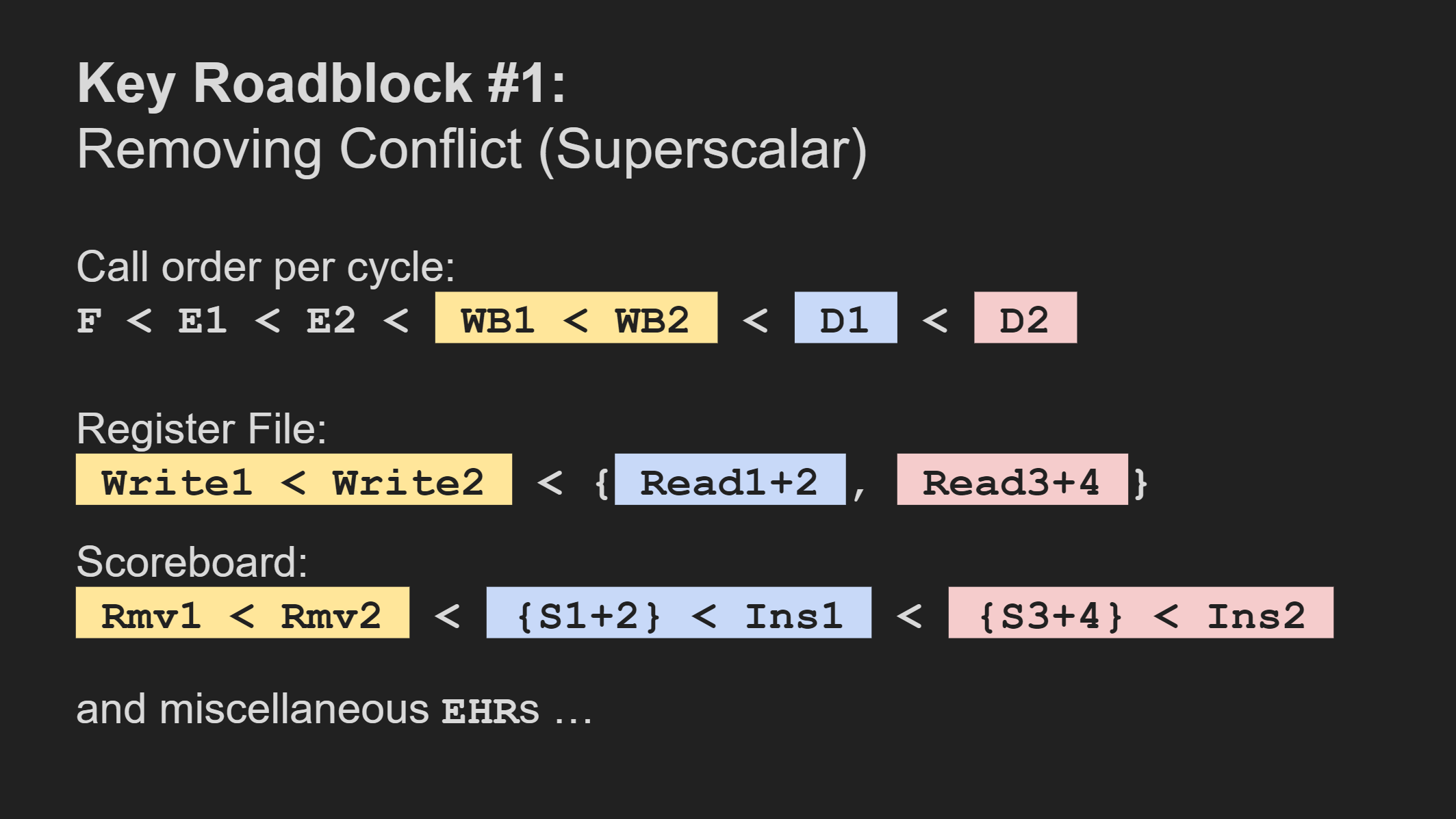
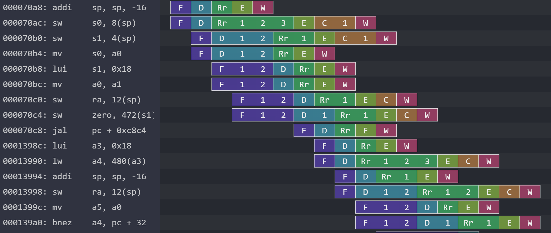
Required scheduling for all 7 rules of our 4-stage superscalar processor to fire simultaneously. The submodule scheduling must be consistent with the top-level scheduling. Note that Fetch has only one rule even for two instructions. I made this slide for my final project presentation for 6.192.

Something that wasn’t immediately obvious was that my processor couldn’t initially execute anything else if we were executing a memory operation. When we execute a memory operation, we dispatch a token both to the next stage and to our memory module. The next cycle, we dequeue this token from both the previous stage and the memory module. In cases where we attempt to issue two memory operations, or even one memory operation and an ALU operation, the next stage can mix up the tokens and mess with our correctness.

The resulting limitation is that when we see a memory operation in RegisterRead, it must go through the execution pipeline alone without either ALU or memory operations next to it. We (much) later solve this limitation when we break up our execution stage into functional units so that we don’t get the memory tokens mixed up.

It was a further but separate issue to optimize these submodules. It’s easy to write an implementation that includes a bunch of unnecessary circuitry, but it shows up in our measurements when the critical-path delay grows ridiculously high. Because maintaining realistic processing was a subgoal, I reduced the amount of unnecessary hardware when I could.

Achieving superscalar processing allowed me to consider implementing more advanced features, like out-of-order processing. It frees up some flexibility when our processor instructions aren’t simply moving in single file.

My superscalar processor with straight-line code. The smoothest sailing there is. Here the code is just initializing our registers to 0.

Before we leave this topic, here’s another observation. We noted earlier that a high issue rate is nothing without a high completion rate, but the reverse isn’t necessarily true. Stalls due to data hazards will often get in the way of being able to issue instructions as fast as we can fetch them, so even fetching one instruction per cycle doesn’t seem to be too terrible for performance as long as everything afterward can keep up.

Despite a low fetch rate, the high completion rate when coupled with the naturally occurring stalls still gives a single-fetch version comparable performance to a wholly superscalar processor.

Out-Of-Order Processing

Nov 12, 2023: It turns out that this part introduces a bug into my processor. The out-of-order commits open the processor up to write-after-write hazards. Read about it in a blog post.

A simple processor typically performs in-order execution. When an instruction has an outstanding data dependency, it usually must stall both itself and all following instructions until the needed data is available. Some of the following instructions might actually be ready to execute, but there’s no hardware that allows the ready instructions to safely bypass the stalled instruction. So, everyone must wait.

We can make a processor faster by adding hardware that allows it to execute instructions out-of-order. Instructions with outstanding dependencies still stall, but instructions that are ready can slide past them. Further, there must be extra logic to make sure that the program is still executed correctly, and the circuitry must be designed in such a way that the increase in critical-path delay doesn’t ruin the increased instructions per cycle.

My processor actually does some out-of-order processing, but it’s such a low degree that I didn’t feel comfortable putting “out-of-order” in the project name. There’s out-of-order processing to the extent that instructions of different types can slide past each other. For example, we can continue issuing ALU instructions even if the memory unit is stalled.

Here’s a particularly flattering example where instructions slide past each other. This fragment comes from our matrix multiplication test where we’re saving values from a hardcoded matrix into memory. Later in the test, we compare our matrix product to this hardcoded matrix to check for correctness. Of course, there’s still major delays because of cache misses. Besides, this fragment is not necessarily a representative portion; it’s one of the few areas of straight-line code in my test suite that also involves interleaved li and sw instructions.

But I haven’t added support for instructions of the same type to slide past each other. There’s no avenue for ready ALU instructions to bypass stalled ALU instructions, nor the same for memory instructions.

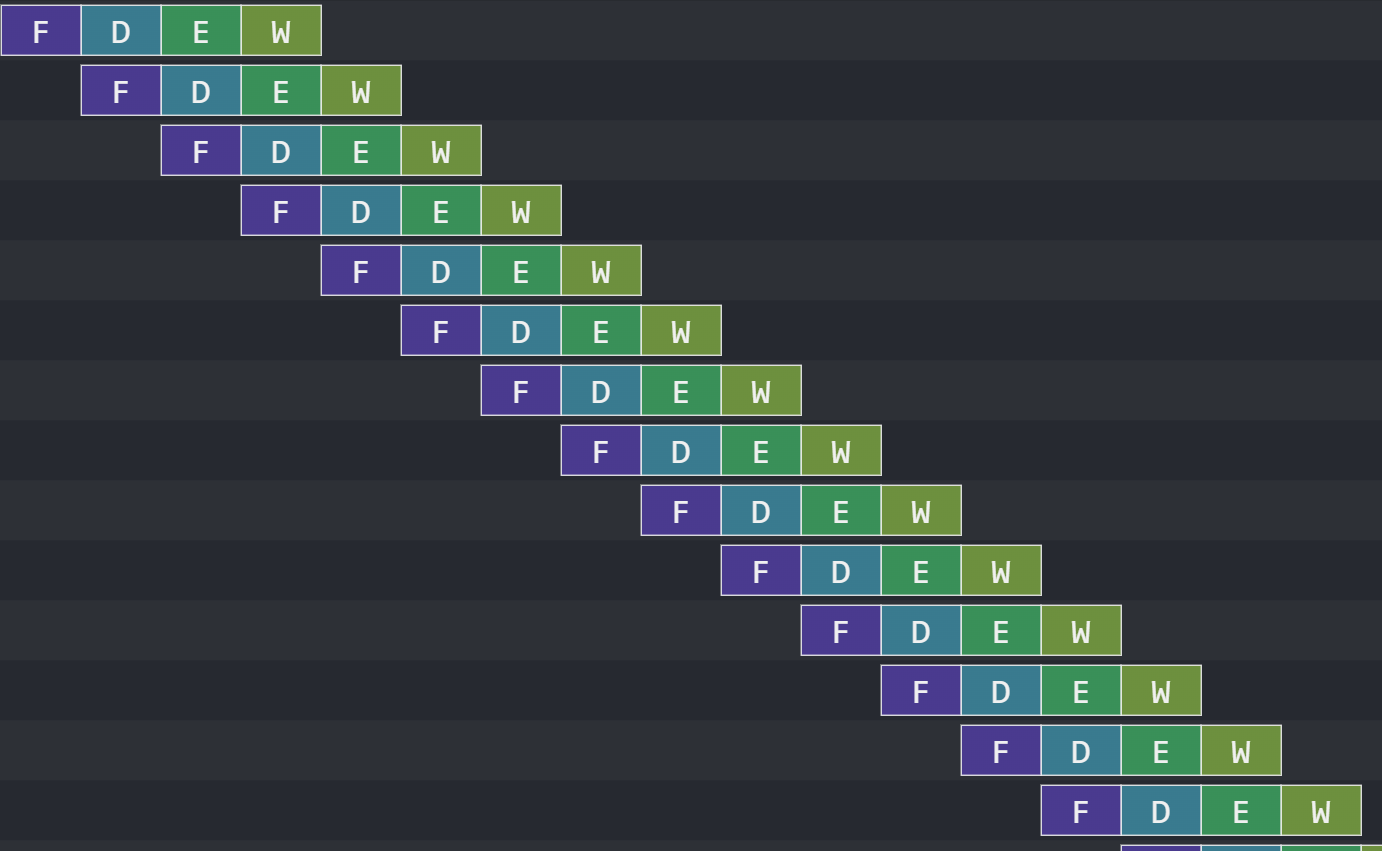
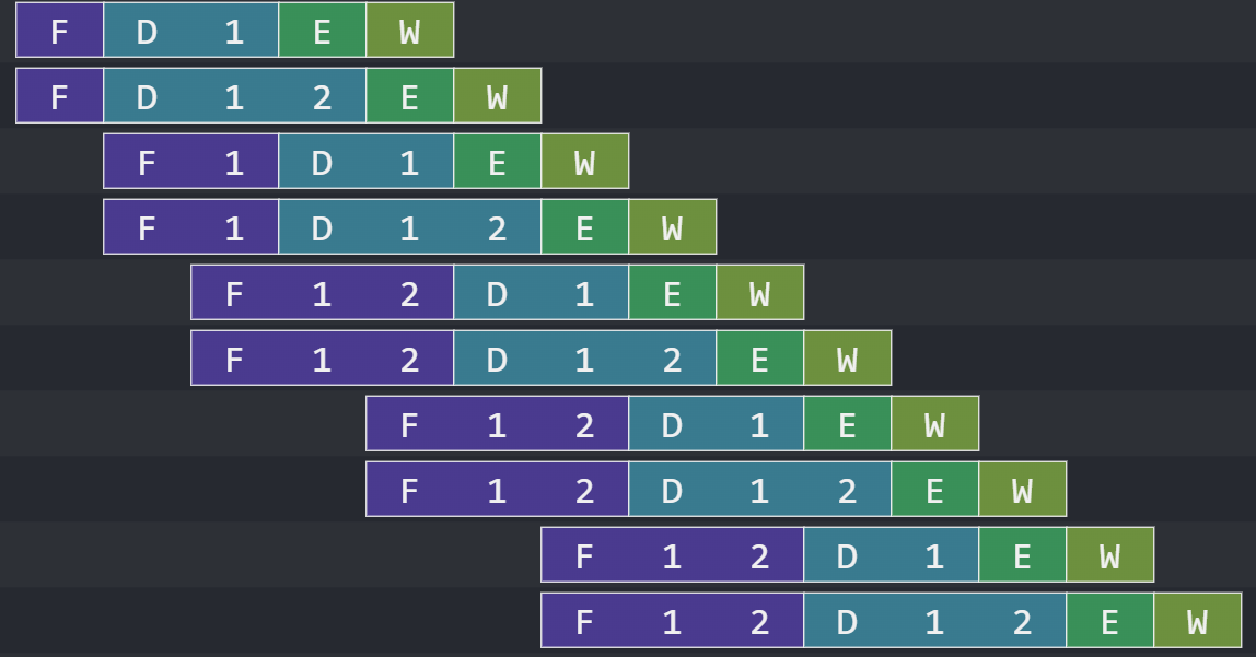
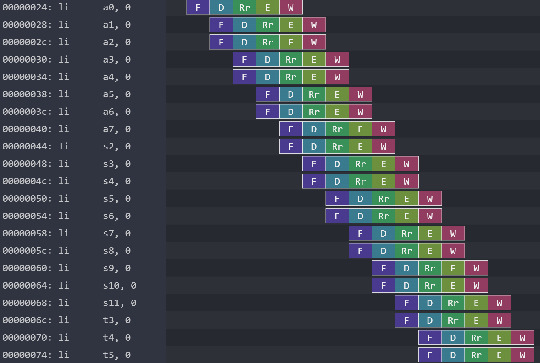
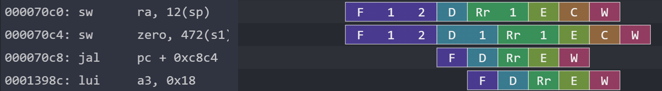
Further, our instruction-issuing component can only see two instructions deep. In the case that the first instruction is stalled, our processor can issue the second without a problem, like in the following example where the second sw is stalled and the jal is ready to go, or the example afterwards where we save to the stack.

The most appealing use case for our limited OOO processing is when we have consecutive memory instructions that can’t issue simultaneously, but we have ALU instructions that are ready to go. Notice how the E blocks are staggered, which is when we begin execution for those instructions.

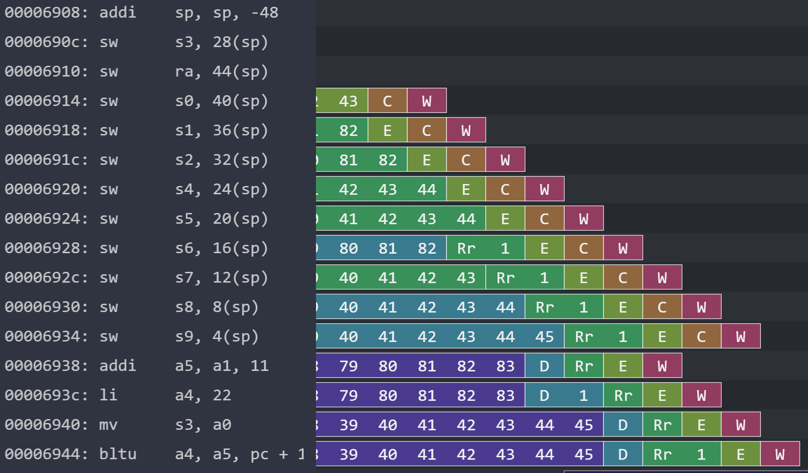
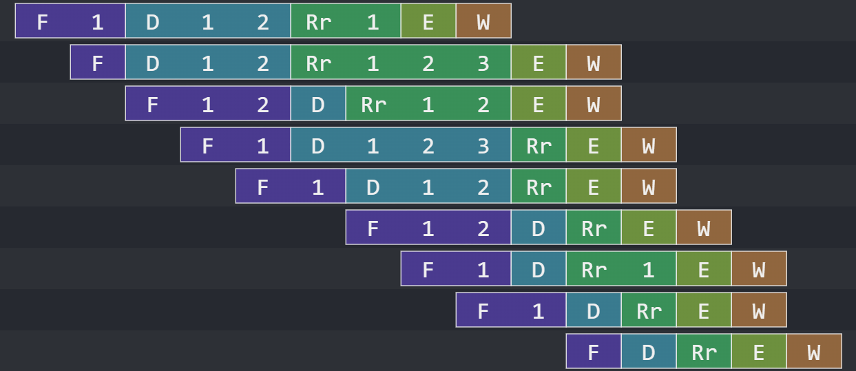
Very slight out-of-order with saving registers to the stack. If more instructions could slide past each other, then we could execute more of the lower triangle before the upper triangle concludes. Also notice how the compiler tries to help us execute out-of-order. It saves s3 first because it’s one of the first registers we need to move a value into, then it saves the rest in order. Putting some distance between dependent instructions allow us to potentially have more instructions in flight. Register renaming can further increase the distance because there’s no true data dependency on s3.

But in cases where two instructions are stalled, we have no ability to see any deeper. One major next step is to write a more sophisticated component that can inspect multiple instructions and dispatch one or two of them. This might use a data structure that behaves like an extractable searchable FIFO, where it can both behave like a FIFO and have elements extracted according to a check for dependencies. This enhancement alone would increase our instruction issue window.

Another thing is that there’s no reordering going on in the processor. Instructions commit as soon as they’re done; it’s just that there’s no problem with it because we only permit ready instructions to issue and we pass operands by value. If we had same-type instruction bypassing, we would probably need to add logic for reordering. We would also need to do the same if we were to add functional units that receive operands by pointer, like we might with some floating-point operations. Reordering also tends to be less big of a deal in RISC-V because we have more general purpose registers than something like x86, so we don’t unnecessarily reuse register names as quickly.

I studied out-of-order processing in the available literature, and I added some of the architectural support for the feature like functional units, but I stopped the project before I was able to produce a wide enough instruction issue window to comfortably call the processor an out-of-order processor.

Still, I thought I made enough progress to warrant naming a section out-of-order processing.

Same image as the preview. A small function call demonstrating some minor out-of-order behavior. ALU instructions and memory instructions are allowed to slide past each other if there aren’t dependencies. There’s no reorder buffer.

A larger function call demonstrating some minor out-of-order behavior. You can also see there’s a bit where we had to flush six instructions.

Literature

This might seem silly, but it didn’t initially occur to me to read the literature on computer architecture. In 6.192, it sufficed to rely only on the lectures and the slide decks to know enough to work on our assignments. We had some materials like the Archbook, but the parts it covered were sufficiently covered in class, and the parts that would’ve been helpful weren’t yet written.

I spent a couple weeks reading up on out-of-order processing, particularly through Tomasulo’s algorithm. There were a few steps I needed to take before I could have the processor genuinely process instructions out-of-order using the Tomasulo’s algorithm reservation station pattern. I did a few of these steps, but not all of them.

It was only on this part that I leaned on written materials. In particular, I read through Computer Architecture: A Quantitative Approach (2017) by Hennessy and Patterson and Modern Processor Design: Fundamentals of Superscalar Processors (2005) by Shen and Lipasti. These are nice and accessible textbooks for a hobbyist or eager learner trying to catch up on microarchitecture design.

It feels a little like a waste that I did so much conceptual studying of the computer architecture principles that go into out-of-order processing without fully implementing it, but I guess there would’ve been no way of knowing to stop short unless I had done that studying. At least it’s in my head now.

Functional Units

I transitioned the processor from a rigid pipeline into what Shen and Lipasti call a diversified pipeline with a rigid start, rigid end, and wiggly middle consisting of different functional units.

FETCH -> DECODE -> REGISTER_READ -> EXECUTE -> WRITEBACK

FETCH -> DECODE -> REGISTER_READ -> { functional units } -> WRITEBACK

This breakup of the formerly rigid middle would’ve allowed me to easily add in, with little glue logic, additional functional units corresponding to new operations, like integer multiply, integer divide, and floating-point operations. These changes represent implementing the M and F standard extensions for RISC-V, which are straightforward but not insignificant tasks. Since I stopped the project, I only have two ALU units and one memory unit.

Additional functional units with their higher latencies would’ve allowed me to better showcase the usefulness of out-of-order execution. Our ALU units only have a latency of 1 cycle and our memory unit only has a latency of 2 cycles. Out-of-order execution would still be helpful without all these fancy operations, but it’s much less dramatic to bypass a stall that would’ve lasted 2 cycles than one that would’ve lasted 20 cycles. The most comparable event in our processor is a cache miss, but we also tend to try and mitigate those by other means.

Branch Prediction

With our superscalar processor, branch mispredictions represent a large penalty because they flush quite a lot of instructions from our pipeline.

An early version of the superscalar processor without branch prediction. The muted color rows represent flushed instructions. Notice that although the angle is steep, implying we get a lot of instructions quickly, many of the instructions are flushed because of misprediction.

Segment of Dhrystone with many misses and large misprediction penalties. Some misses are unavoidable if it’s the first time our program has seen them, but misses our program has encountered before should be used to inform future speculation.

My branch predictor only uses a 32-line branch target buffer (BTB). I have a rather tight control loop in my processor because I confirm control flow in RegisterRead before instructions issue. The predictor would become even more important if I had a bigger delay before confirming control.

Matrix multiplication routine on superscalar processor with very effective branch prediction on a small loop.

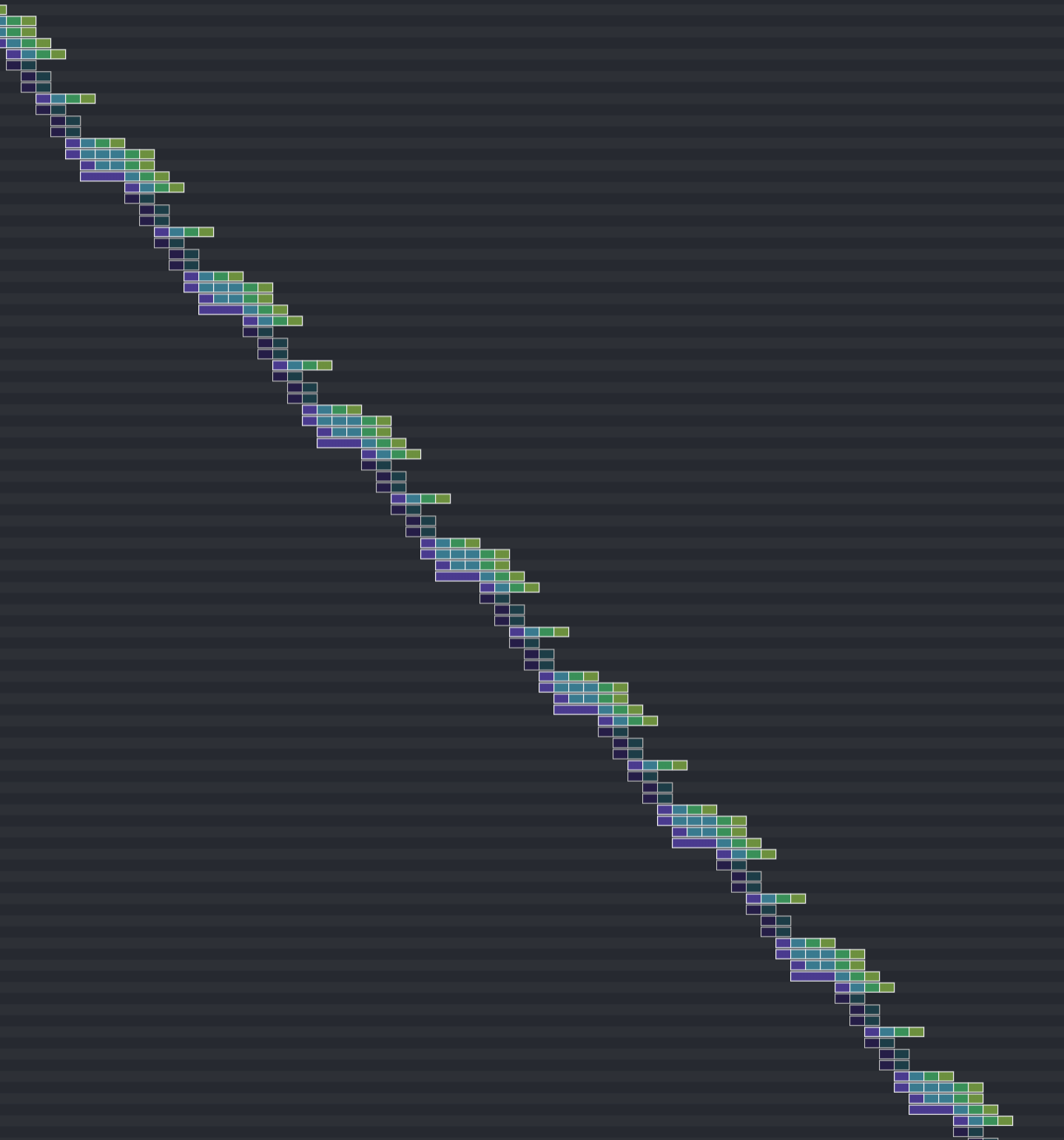
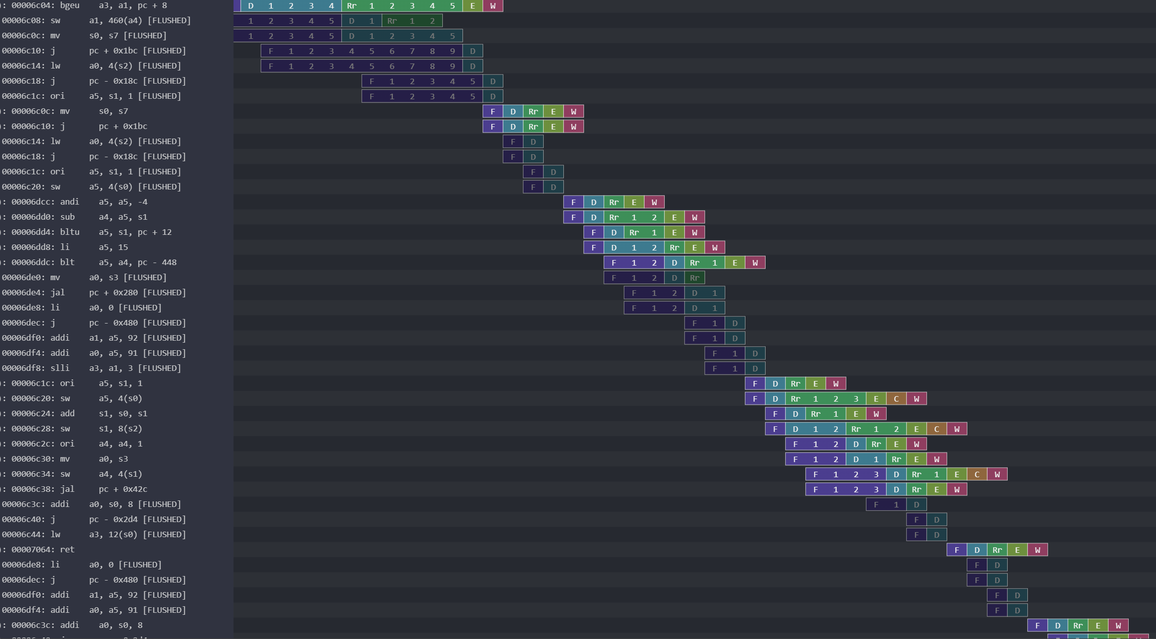
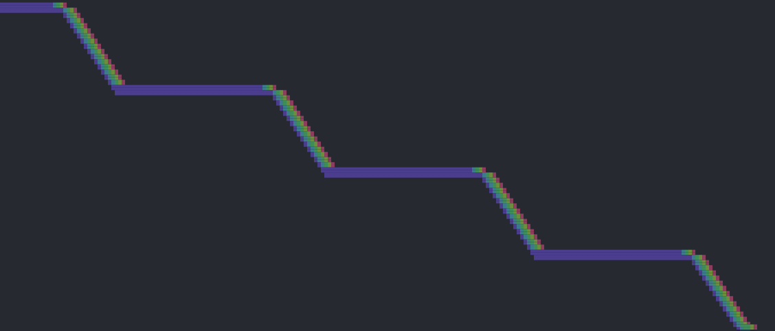
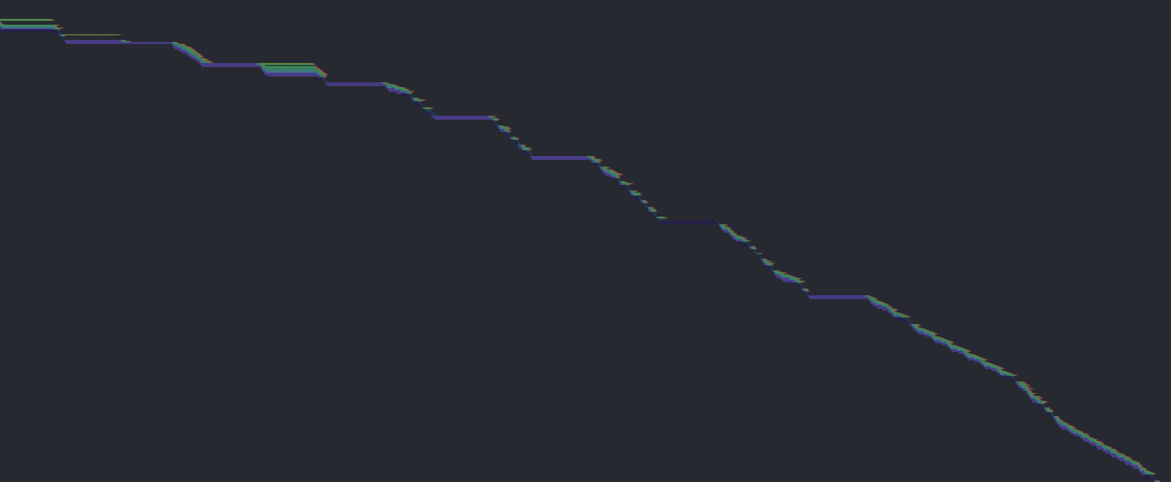
Let’s do some comparisons between our BTB-based predictor and a basic predictor that always assumes no branch (pc + 4).

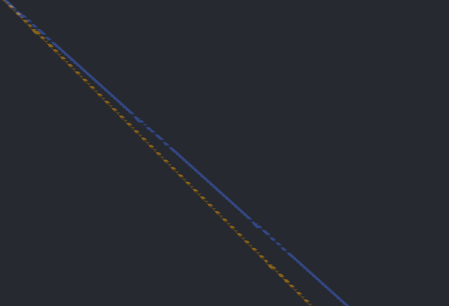
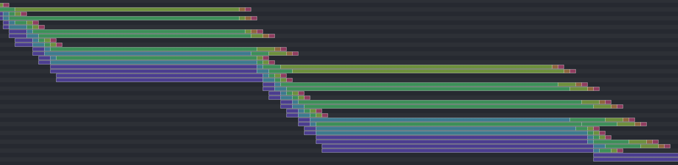
These two overlaid runs differ only in the branch predictor used. The blue uses a BTB, whereas the orange uses the basic predictor pc + 4. Notice that the basic predictor has a much steeper slope, which might imply a higher number of instructions per cycle. But what happens if we remove the flushed operations from the chart?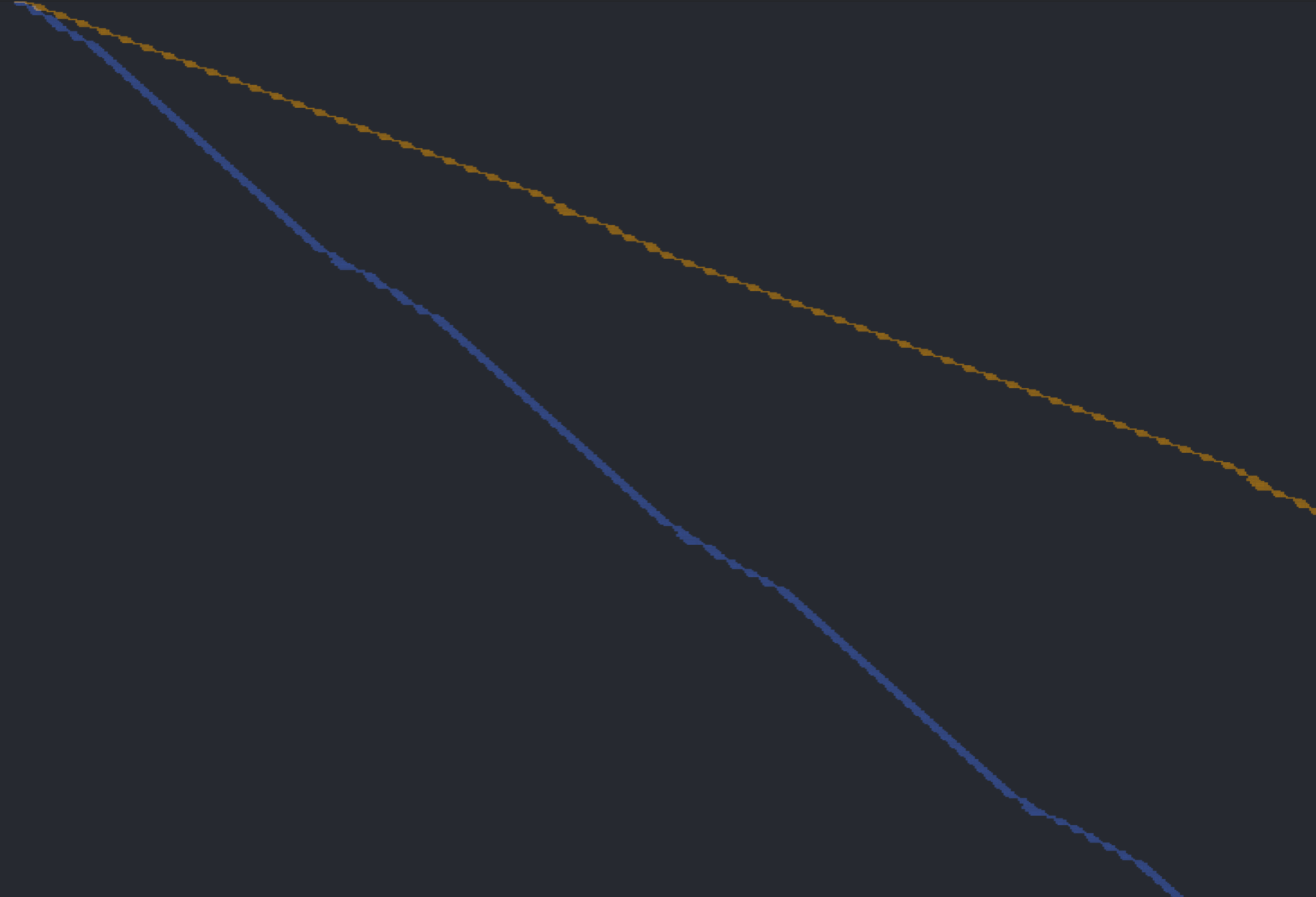

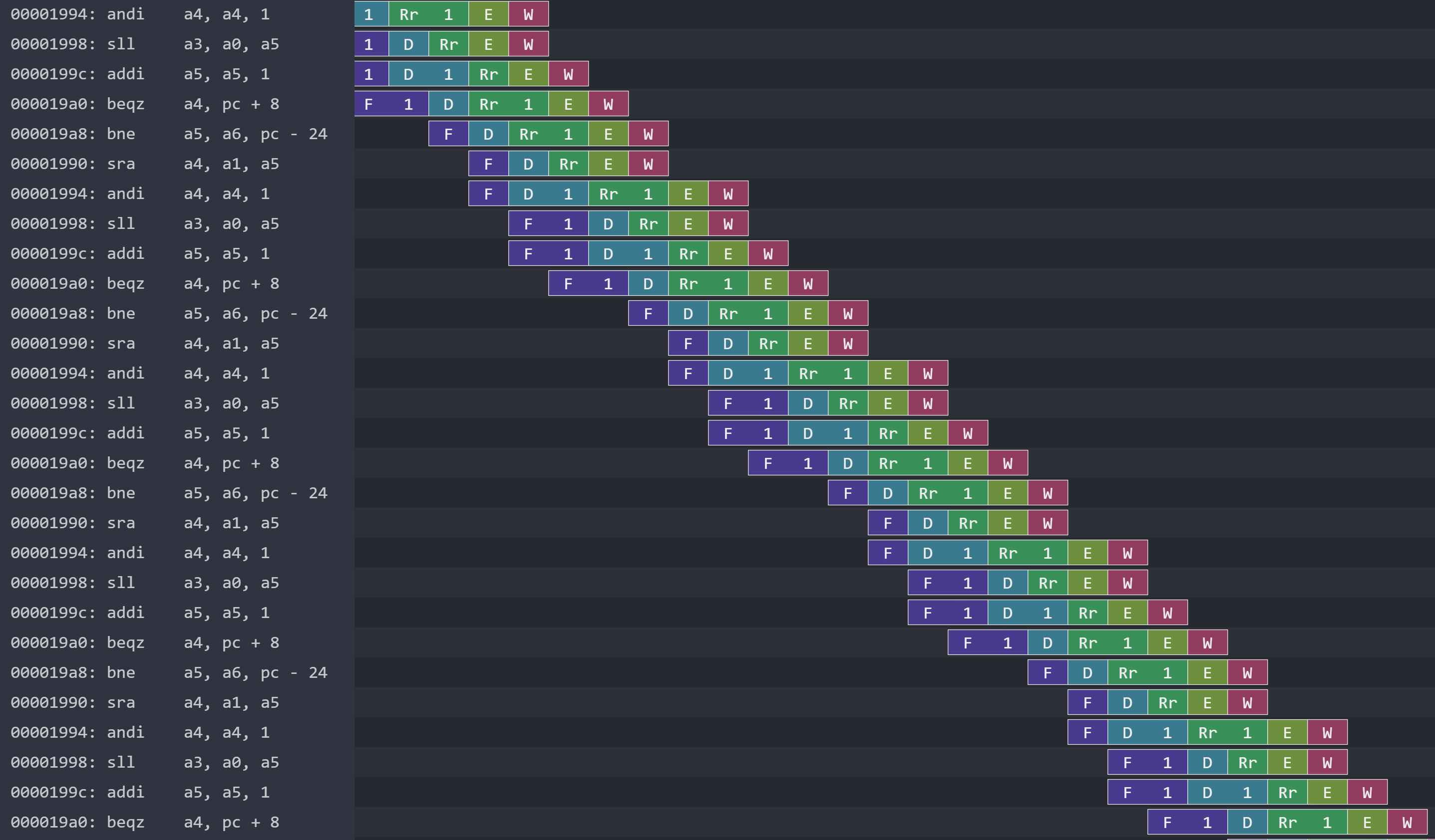
This is the same pair of runs as the previous figure, but here flushed operations are hidden. Both lines have flattened a bit, but the transformation is much more pronounced for the basic predictor (orange) because so many of the instructions were flushed.

The instructions-per-cycle (IPC) for the BTB is 1.0632, whereas the IPC for the basic predictor is 0.5256. Less than half!

Of course, matrix multiplication without the M extension is a particularly flattering test case because of the high frequency of very short, very tight loops from repeated addition. Other tests are likely to show more modest improvements.

If I worked further on the processor, I would plan to add in a large branch history table (BHT) and a return address stack (RAS). Their usefulness would be more obvious with larger programs that involve lots of possible branch targets and lots of deep function calls, respectively. I don’t currently have benchmarks set up that display that kind of behavior, but I would try and get some.

The added logic might, because of critical path constraints, encourage me to spread out the control calculation depending on when information becomes available. For example, I might precompute addresses that don’t require a register read so that there’s less computation to do during that stage.

Measuring Predictor Performance

Debugging a branch predictor requires careful logging and close inspection. A faulty branch predictor simply causes our processor to run slower, but it usually doesn’t cause the processor to produce incorrect results. That’s why it becomes important to have ways of checking the predictor’s behavior. This sort of debugging was how I discovered a major bug in my BTB where I was using only a quarter of the lines. When I was using the pcs as keys into the buffer, I didn’t chop off the two least significant bits, which were always zero.

Although in practice, I mostly measured the performance by eyeballing the debug output and seeing on the Konata visualization whether we had any predictable branch misses. A more rigorous approach may involve analyzing the trace of executed instructions.

Logging for the branch predictor (just a branch target buffer) with moderate performance on a part of Dhrystone.

The branch predictor with good performance on a part of Dhrystone.

The branch predictor on a very tight matrix multiplication loop with excellent performance.

Cache Improvements

The base for my improved caches was my cache implementation from class, though I had to upgrade it from the toy example into a more realistic (so I’m told) 128-line 16-word-per-line L1 cache. For the superscalar design, I split my cache into one instruction ReadOnlyCache and one into a normal data Cache.

Part way through the project, I also pulled the caches onto the chip itself for synthesis. The move increased both synthesized area and delay because we just didn’t count them before. But I think it allows me to make stronger claims about the practicality of the processor, since the cache isn’t just sitting on the sideline. Part of my motivation for pulling in the caches was reading about superpipelined processors in Hennessy and Patterson, where the cache constituted a big enough delay where they had to pipeline steps within the cache. It would feel weird if I didn’t know whether my caches bottlenecked my design.

If I was to continue working on the caches, I would seek to make the data cache non-blocking upon misses, and maybe make it two-way associative too.

Store Buffer

An early improvement I made was implementing a store buffer. When our cache receives a load, our processor tends to stall until it receives a response. So, it’s important that we prioritize loads over stores. This is even more true when we consider that storing in our cache requires two cycles (one to get the cache line, another to modify and save it back).

With our store buffer, when we receive a store request, we put it off to the side and pretend it hits. Next cycle, we see whether we receive another request.

• If we don’t receive a request, we begin processing the oldest store buffer entry.
• If we receive a store request, we add it to our store buffer but we begin processing the oldest store buffer entry too. This is so our store buffer doesn’t fill up while our cache internals lie idle.
• If we receive a load request, we process that immediately.

The idea is to keep our cache internals open for loads. It also allows the cache to continue background work while our processor is busy processing ALU instructions, spreading out the computation.

This particular design isn’t necessarily optimal; once we start processing a store it will take another cycle to finish, so having no request this cycle and a load request next cycle will make the load wait. An improvement requiring more hardware could be allowing a two-cycle store to be put on hold in the case of an incoming load request. But for the hardware complexity, it’s not too bad. This design was already difficult enough to debug.

My data structure that implements the store buffer is also not optimal, and I discuss it later in optimizing submodules. My inefficient implementation causes the critical-path delay to grow too much with respect to the number of entries.

Prefetching

Each instruction cache line fill takes 16 words of instruction. With straight-line code, superscalar processing consumes 16 instructions in only 8 cycles. Our L1 cache model however has a miss penalty of 40 cycles. Prefetching allows us to have a better ratio of runtime versus cache miss time for straight-line code.

The prefetch functionality I implemented doesn’t actually ensure continuous fetching without misses for straight-line code. All it does is whenever we fill an instruction miss, we also fill the next line. There isn’t much additional cost because our main memory (out of the scope of the project) is internally pipelined. This lazy approach does penalize us for straight-line code, but because straight-line code constitutes such a small part of our benchmarks, I didn’t worry too much about it.

A slightly more sophisticated prefetcher would maintain some distance to when our next “predicted” cache miss would be so we would never have a cache miss for straight-line code. At peak performance, we would need to stay five lines ahead. An even more sophisticated prefetcher may even look ahead for control flow instructions and prefetch the instructions at those targets, just in case.

Our prefetcher just fetches two lines of instructions instead of just one. Here is a contrived example meant to illustrate the limitations when we have more than 32 consecutive instructions of straight-line code.

More aggressive prefetching requires additional hardware and might even reduce performance. We could prefetch more aggressively if our cache was non-blocking on misses and if it had some associativity that protected against evicting our current stream of instructions. For a project where every feature cost me some development time and where the goal was out-of-order processing, I went for the first approximation of prefetching.

Our prefetching makes particular segments of code (like our prelude) smoother since it’s slightly more than 32 instructions of straight-line code, but I didn’t rigorously check how effective it is overall. An appropriate step would be to take some larger benchmarks and check for the number of instances when we get more than 16 instructions without control flow interruption, and do the same for 32 instructions, 48 instructions, etc. to see how much prefetching is actually necessary compared to the overall runtime. When I was tuning the prefetcher, I found that my benchmarks benefited from prefetching one line, but not from prefetching any more. I believe the issue was that my direct-mapped instruction cache was getting useful lines knocked off due to conflicts with prefetching.

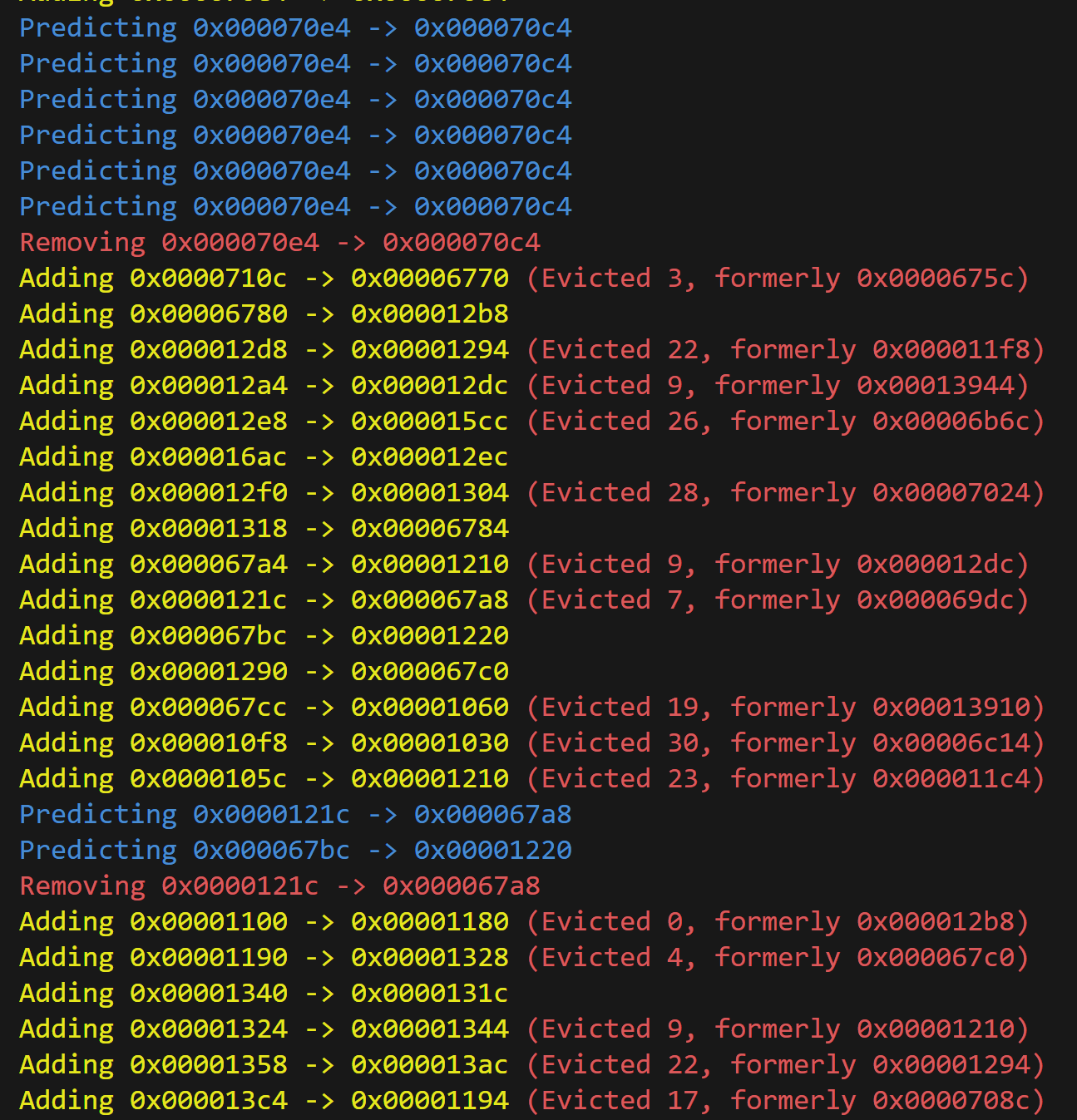
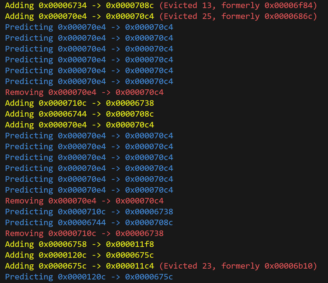
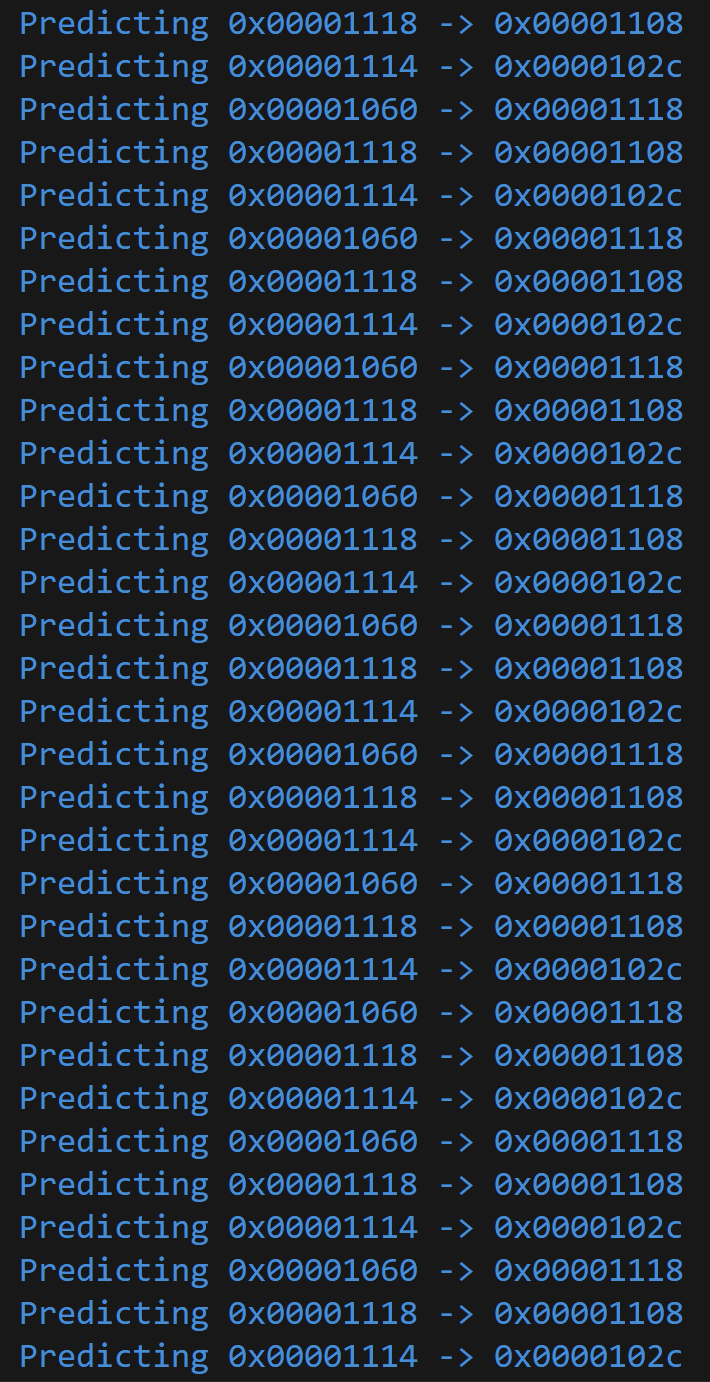
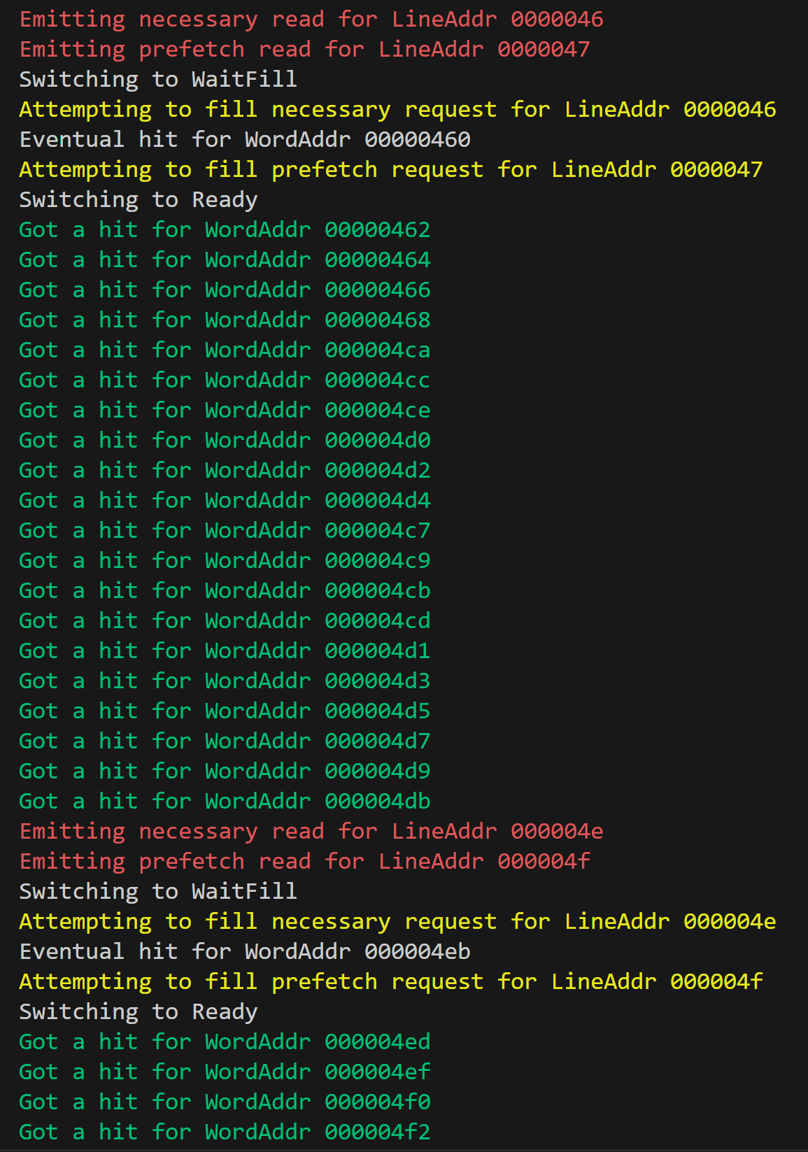
Because I couldn’t rely on the Konata visualizations for isolating and debugging the prefetching feature, I had to use logging in the terminal. I’m quite pleased with using colorful messages; it was my first time doing it.

Logging for the instruction cache internals, including fills for misses and fills for prefetching.

Notice that prefetching has some relationship with branch prediction, in that they work together to reduce the number of instructions we need to flush.

Infrastructure

Not every task had direct implications for the processor performance. Sometimes I would spend some effort on building infrastructure or instrumenting my processor in a way that would make development easier or more robust.

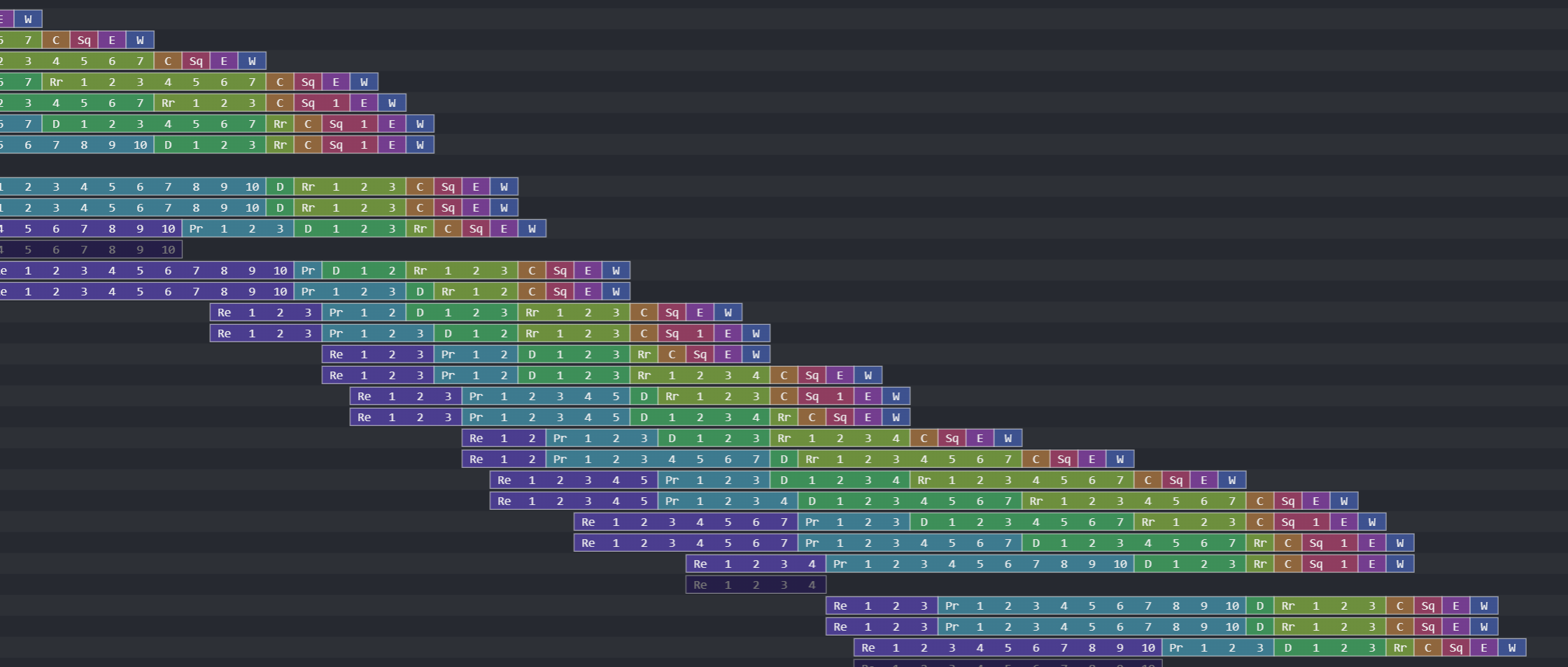
Konata

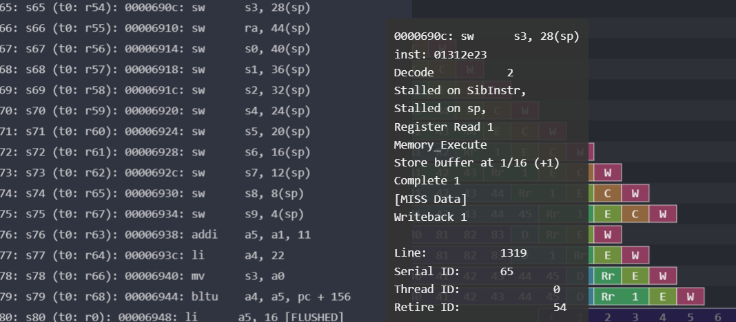
Just seeing test results in the terminal isn’t quite enough for checking in on how the processor is working. One tool that I really enjoyed using was the Konata pipeline visualizer, which was introduced to me in the 6.192 class. I had the fortune of already having a skeleton for logging from class assignments, but I made major changes to the instrumentation so the logging would produce useful annotations for debugging my processor.

The only other pipeline visualizer I’ve ever used was in 6.004 (now known as 6.191), where the visualizer was just black-and-white ASCII printed out in the terminal. I’m also aware of more sophisticated terminal-based visualizers like the gem5 O3 Pipeline Viewer. It’s now 2023, and I think we deserve tools that have pretty output like Konata. This tool was indispensable for working on this project. I used many of the pipeline visualizations as illustrations in this report.

Konata logs allow the developer to add annotations to particular instructions both upon mouseover and on the side. Here the mouseover annotations tell us which particular stages the instruction goes through, reasons why the instruction stalls, and other information like how full the store buffer is.

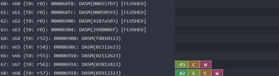
This is what the annotation looks like before processing. For the side annotations, I like to have instructions in a readable assembly form. For that, I use an external tool from the RISC-V software suite called spike_dasm. I just log each instruction with the DASM() marker, then I use the tool to process the entire Konata log file line by line. Before I discovered this tool, I was using a hacky solution of duplicating the decoder logic and having it output strings for the processor itself to write to the log. It was both a pain to maintain and incapable of complex decoding like detecting pseudoinstructions.

Other features I appreciated and that you might’ve seen in previous sections are the grayed-out coloring for flushed instructions, the colorful display, and the ability to zoom in and out at will. In some instances, I would also run comparisons between different pipelines, like for the branch predictor section.

Automated Benchmarking

One of my very first acts in the early summer was to write scripts to automate repetitive tasks. That might be a no-brainer for more seasoned engineers, but it wasn’t really something I had much exposure to in school. For most of my classes, we would have infrastructure already be built for us by the course staff. But because implementation efficiency wasn’t a priority in 6.192’s assignments, there wasn’t any prebuilt infrastructure on checking how well our processor was doing as long as it worked.

Throughout most of the project, I kept track of the critical path delay using the synth tool in Minispec. Behind the scenes, it compiles my BSV to Verilog and then synthesizes that with the yosys framework.

My delay usually hovered between 900 to 1200 ps. I would multiply this delay with cycles per program (as per the iron law of performance) to see how my processor was doing.

Because I was going to be running the same tests repeatedly and I wanted to track performance over time, I decided to write a set of Bash and Python scripts that would log my performance after successfully passing all the tests. It would perform synthesis, do the iron law multiplication for each test, and compare the performance to a set of reference numbers from previous runs.

I wouldn’t say the scripting was too difficult, but it did require me to do some fumbling because it was the first time I wrote a Bash script with more than a few lines. It was all pretty much just trying to figure out what I would ordinarily want to call via the command line, figuring out how to make it pretty, then figuring out how to make the script do it.

Here’s an example log from my last commit:

Benchmark summary

mkpipelined
Gates: 216050
Area: 289505.76 um^2
Critical-path delay: 1160.39 ps (not including setup time of endpoint flip-flop)
Critical path: fu2w_enqueueFifo_register -> $techmappc_unit.predictor.$0buffer_1[65:0][8]

Cycle counts [first is Dhrystone]
781 [906 ns] (96.3%)
432 [501 ns] (121.6%)
432 [501 ns] (121.6%)
432 [501 ns] (121.6%)
432 [501 ns] (121.6%)
432 [501 ns] (121.6%)
829 [962 ns] (113.4%)
673 [781 ns] (109.7%)
13801 [16015 ns] (142.1%)
35853 [41603 ns] (127.2%)
17773 [20624 ns] (117.1%)
Notes:
Unblock rules from each other. Still in-order issues within instruction types, but OOO issues across;
i.e., a memory instruction can be passed by an integer instruction, and vice versa.

There's still some rule shadowing that I should factor out eventually, but it doesn't affect the correctness
or performance. It's just technical debt for debugging.

FINAL COMMIT

Looking at this log reminds me that the BSV ecosystem is missing good out-of-the-box critical-path analysis for synthesis (at least to my knowledge). I get the start and end points of the critical path, but the names get mangled so I can’t really see what structures are involved in the middle of the critical path. Careful reasoning can reveal the most likely candidates, which is what I did, but that requires the programmer to do some work that could’ve been delegated to the machine.

Dhrystone

The main benchmark I used to measure performance was Dhrystone. I used the amount of time necessary to run one Dhrystone as the main number that sums up my processor’s performance, which I got by multiplying cycles per Dhrystone by my synthesized critical-path delay.

Konata was useful for looking at the Dhrystone runs and thinking about where to focus next. This was also the only test I had that really used stack saving, since the benchmark was designed to simulate real programs (at least back when it was written).

I made this line chart in Excel using the numbers from my automated logs. Each point represents a different version in the development process. The leftmost point (1177 ns) represents the first run I started tracking Dhrystone performance. The time then goes down when I take out the unnecessary pipeline stages. The minimum during tracking was 776 ns, right after fixing my branch predictor from being de facto 8 lines to 32 lines (decreasing instruction cache misses). It goes back up again to 906 ns when I add in overhead for functional units in preparation for out-of-order processing, but I end the project before I’m able to bring it back down again.

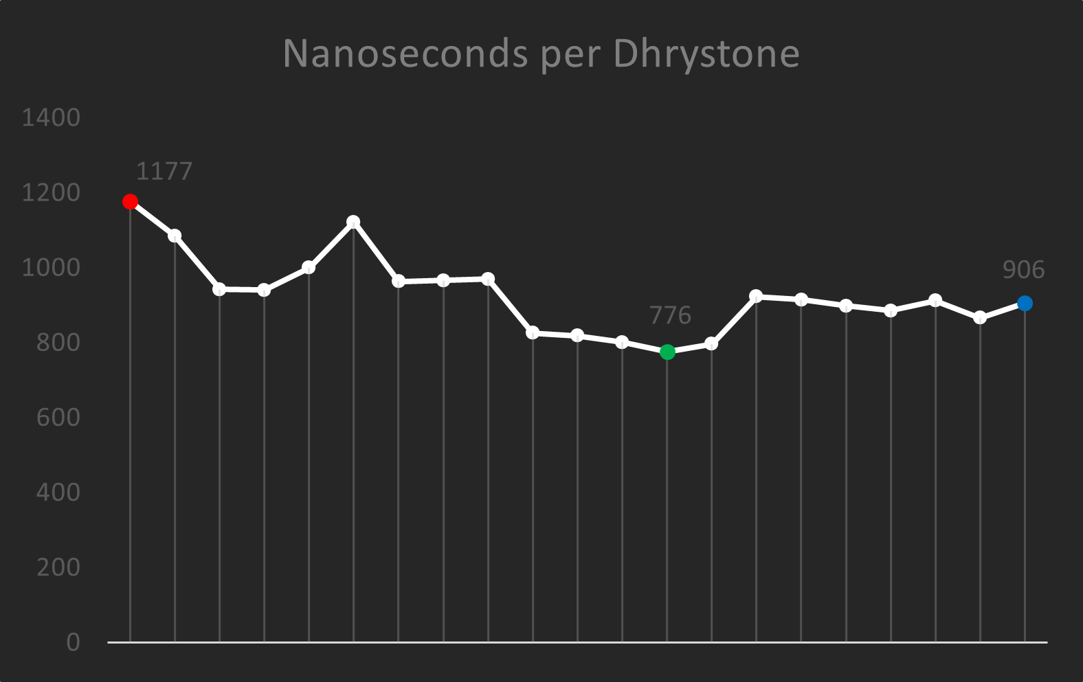
A common criticism of Dhrystone is that it’s too old (40 years old!) and is no longer representative of ordinary computing. I think that’s probably true. The issue was that I had difficulty finding benchmarks that could easily run on my processor. I cobbled together the Dhrystone benchmark as a stopgap to measure the performance of my processor against previous versions of itself. It’s about balancing the need for infrastructure with the need for features.

I looked at a heftier repo of RISC-V benchmark tests from the RISC-V team but they don’t work off the shelf. I spent a couple days trying to configure it, but it seems like they require at least the Zicsr extension to run. Going out of my way to implement the extension felt like too much effort taken away from actually implementing processor features.

I also looked at the SPECint suite of benchmark tests. Those tests are a pleasant mix of computing tasks that we might see as more representative of computing in the 21st century. But I didn’t have a license to use the suite, nor did I have the desire to shell out the money necessary to buy one, especially since I was doing this project as a hobbyist.

RISCOF Support

RISCOF is a framework maintained by the RISC-V team for testing a processor design for compliance with the RISC-V standard. In 6.192, we ran integration tests that implied our processor followed the standard, but I figured using an official tool would be useful for future debugging since I was going to be making major changes to the processor design.

Getting RISCOF to run wasn’t the hard part. I wrote the little Python plugin as the RISCOF team had prescribed to allow the framework to run my processor. The main issue had to do with instrumenting my processor to output a test signature that RISCOF could then compare to the reference signature.

By default, my processor didn’t log any of its state (memory or registers) outside of the Konata logging. Rather, the only way we got any information out of the processor was through its MMIO operations, where the processor saved to a hardcoded address that actually corresponded to the BSV stdout stream.

Because I didn’t have access to any control/status registers due to not having implemented the Zicsr extension or anything like it, I configured my processor to dump its memory with a combination of hand-written assembly (to tell the processor what addresses to look at) and some custom RISC-V instructions using the HINT instruction slots.

My protocol was to issue slti x0, x0, imm instructions, which my processor would parse as requiring to read a0 and a1 and run an operation corresponding to the value of imm. I only implemented two of these (which I call system instructions): one for halting (imm = 0) and one for dumping (imm = 1). It was a little hacky, but it produced the signatures I needed to verify that my implementation was correct.

Once I got RISCOF to work, my processor, as expected, immediately passed all tests for the target, which was the plain rv32i ISA.

The point of configuring for RISCOF is that I wanted to have useful tests for later implementing extensions, like the M and F extensions. Those extensions aren’t necessarily required, but they would’ve been nice to have to better show off out-of-order processing. Their higher latencies dramatically increase the relative benefit of out-of-order. Of course, I didn’t end up finishing out-of-order processing and I didn’t end up adding in these extensions.

Minor Components

There were some parts of the development experience that I would like to discuss, but weren’t major enough to warrant entire subsections in the major components section. These tend to be the less visible features, either because their changes were reversed or because they literally don’t reflect in the pipeline visualization. I discuss them briefly below.

Appropriate Pipelining

I had a brief phase in the development process when I thought I should just introduce as many pipeline stages as possible. Spread it all out; isn’t that what people mean by having deeply pipelined processors?

Well, that approach works best when there’s actually enough computation going on at each stage. For my processor, there simply wasn’t much going on at each stage to warrant further pipelining. A variation on the classic RISC pipeline was sufficient for all the hardware I was adding. Additional pipelining was simply premature optimization especially since I hadn’t truly implemented out-of-order processing. There would always be time to rebalance stages later.

Wow! Pretty visuals, but there are so many unnecessary cycles per instruction.

When I added these additional stages, performance ultimately suffered due to the increase in cycles per instruction. I cooked up stages that I had no reason to add in, like one just for predicting and one just for squashing. Further, these didn’t actually increase the number of instructions in flight all that much. Despite the higher number of stages, later instructions were often stalled a long while.

When I came to my senses, I removed the excess stages. Having a simpler pipeline also allows me to reason more easily about out-of-order processing. Deeper pipelining isn’t off the table, but it should be deferred until at least there’s enough unbalanced critical-path to make splitting a stage an obvious choice.

Optimizing Submodules

To maintain a sensible critical-path delay, I would sometimes need to optimize the data structures that underpin some of the processor’s modules, like the register file or scoreboard.

For the very first implementation of a data structure, it’s usually a good idea to just focus on correctness. One of the main building blocks for my basic implementation of the register file, scoreboard, and other data structures was the BSV module corresponding to ephemeral history registers (EHRs). These enable what seem like multiple sequential reads/writes to a register in a single cycle. They allow for easy implementation of bypassing and communication between rules firing in the same cycle.

But EHRs are expensive. The issue is when not all these ports are needed. You can imagine there can be significant delay when we require every register in the register file to accommodate for several (simulated) sequential read/writes. To optimize the register file, I recognized that we only needed to have two write ports for the whole register file. To facilitate bypass without a whole extra layer of EHRs (which is what my basic implementation used), I kept the internal representation of the register file as plain registers, then only made the write ports into EHRs, which gives us our bypass functionality. Then at the end of each cycle, these EHRs would have their values written into the register file, emptying out the ports for next cycle. This stage is what 6.192 often referred to as canonicalization.

A next step might be to improve the implementation of my SearchFIFO. The data structure underpinning my store buffer has an implementation sufficient for 8 entries, but the design becomes impractical for a higher number of entries. I used a modification of MIT CSG’s SearchFIFO, but a tree-like implementation would probably be more efficient for my purposes. Once I improve the data structure enough, I may also be able to use an augmented version of it for my issue buffer for out-of-order processing. Something about smart data structures and dumb code working better than smart code and dumb data structures.

More careful design of my other data structures would probably also improve my critical-path delay.

Appendix: Background

Most of my undergraduate education has been software engineering with some focus on computer systems and performance engineering. I had only taken two classes that had anything to do with hardware design. The first was 6.004 (now 6.191), a survey class of computer systems that had an optional final project to co-optimize our pipelined processor implementation and our quicksort RISC-V implementation. I really enjoyed that project, so I took what was presented as its sequel, 6.192 (formerly 6.175).

6.192 is an advanced undergraduate elective at MIT covering modern computer architecture techniques. When I took it Spring 2023, it had been 5.5 years since the last time it had been offered back in 2017 as 6.175 and half the material was new. Part of it was a review of a classic 4-stage RISC pipeline and cache design, and part of it was a survey of intermediate topics in computer architecture.

We discussed superscalar processing, branch prediction, vector processing, hardware acceleration, cache coherence, and multithreading. These topics would later play a role in the final project, which would later serve as the base for this project.

A thread that ran throughout the class was being able to quickly prototype a simulable, synthesizable, and efficient circuit from a high-level hardware design, so we had been implementing some of the structures we discussed in class. For example, one assignment was to pipeline a given 4-stage multicycle RISC-V processor, and another assignment was to implement a simple cache. Other assignments implemented modules that would find their place in a more complex processor (completion buffer, butterfly shuffler, etc.), but our processor was simple enough that we didn’t need these components. My instructor Thomas oriented the materials so that everything we did was reflective of concepts employed in real processors.

My impression is that the focus on rapid verifiable prototyping set the class apart from conventional hardware design classes. It wasn’t exactly just high-level computer architecture in terms of making models of the design space, and it wasn’t exactly just RTL implementation. This hybrid work (which is what I was led to believe: hybrid work with respect to what usually happens in industry, at least the bigger shops) was what the instructors labeled constructive computer architecture. We were taught in Bluespec SystemVerilog, in part because of its higher level of abstraction serving their pedagogical goals better, and in part because the class’s lead instructor Arvind had co-founded Bluespec.

I haven’t yet had serious direct exposure to Verilog or SystemVerilog or other mainstream HDLs. I say “direct” because BSV itself compiles to synthesizable Verilog and has syntax derived from SystemVerilog. I don’t doubt my ability to pick up these HDLs; we just didn’t use them in the classes that I took. It’s BSV’s higher level of abstraction, but still within range of synthesis, that made it practical for us to study the breadth of architectural techniques that we did.

The final project for the class, which we spent the second half of the class on, was to implement some of the advanced architectural features we discussed in class. I selected superscalar processing to work on. Before implementing anything, we also needed to upgrade our simple cache implementation into a realistic L1 cache implementation and integrate it into our processor. That integration ended up taking much of the class, including me, more time than the instructors had planned, so not everyone was able to make it very far with respect to the advanced features.

For my final submission for the class, I was able to do a buggy implementation of superscalar processing, but not much more. After the class was over, I still wanted a deeper dive into computer architecture so I continued the project, both to complete superscalar processing and to add further improvements, and that is what you see here today.

I’m not super sure what’s in my future. If it’s more computer architecture, I feel like this project gives me some useful exposure that helps make up for my lack of conventional hardware design classes. If it’s computing outside of computer architecture, I feel like having some better understanding of processors will help inform my work much in the same general way that having studied algorithms does. After all, it’s what our programs run on.

If you came directly from the overview, you can jump back to right after the overview.

Appendix: Detailed Timeline

I’m not sure how useful this timeline is to an outside viewer, but I assembled this from my notes and git commit history as an aid to help me write this project write-up. Here it is for your viewing pleasure.

Spring 6.192 Class

• 2023-04-13: Begin class final project. Start with working 4-stage pipelined scalar processor with magic memory and toy caches. We made these components as earlier homework assignments. The aim for the project is to widen the processor to a two-issue superscalar processor connected to realistic L1 caches.
• 2023-04-21: Write script for translating 16-bit hex to 512-bit hex in preparation for connecting our caches to the processor, since we need to preload our memory. I shared this tool with the class.
• 2023-04-22: Complete realistic cache implementation with 16-word blocks.
• 2023-04-27: Connect instruction and data caches to processor core.
  • Pipeline instruction cache to take requests and serve responses in same cycle.
  • Extend our testbench and data cache to accommodate byte and halfword stores.
• 2023-04-28: Complete working two-word Fetch to feed superscalar pipeline.
• 2023-05-01: Basic implementation for superscalar Scoreboard and 4R2W Register File.
• 2023-05-01: Complete working simultaneous Decode_1 and Decode_2.
• 2023-05-02: Fix scheduling conflicts for all simultaneous stages; not yet fully correct because of hazards with memory tokens.
• 2023-05-04: (Meta) Clean up build scripts to use bash instead of weird Makefiles.

Early Summer

• 2023-06-13: Complete full working superscalar implementation (but with lots of branch mispredictions and cache misses).
• 2023-06-14: Major infrastructure improvements from writing bash and Python scripts for automated testing and logging, including comparison to baseline performance. Measures both cycles and critical-path delay from synthesis.
• 2023-06-15: Implement instruction prefetcher to fetch the next line. Increases our superscalar performance due to reducing predictable instruction cache misses.
• (2023-06-16): Refactoring, encapsulation, and additional logging (with color!) for easier debugging.
• 2023-06-17: Implement initial branch predictor with branch target buffer (BTB) (16 lines but effectively 4 lines because of an implementation error with pc) to significant performance benefit.
• 2023-06-18: Change implementation of our data structures to more efficient ones (less area, less delay)
  • 4R2W Register File to one with sensible bypasses, rather than additional EHR ports.
  • Scoreboard without redundant ports.
  • AddressPredictor to be truly conflict-free with prediction and updating
• (2023-06-20): Add automated critical path * cycles analysis to benchmark tool.
• 2023-06-22: Begin integrating RISCOF support into our processor.
  • Change our test building Makefile to use an elf2hex that directly outputs 512-bit lines. Deprecates our earlier 2023-04-21 script and class-provided elf2hex.
  • Set up RISCOF to execute our prelude before each test.
• 2023-07-03: Complete dump capability for our processor to create a fully RISCOF compliant signature file from running a test using +riscof plusarg. Now fully integrated with RISCOF.
  • Dump uses a series of custom “system commands” implemented via the RISC-V HINT instruction slti x0, x0, code, where halt uses code = 0 and dump uses code = 1.
• 2023-07-05: Minor fixes
  • Change our Konata logging to use spike-dasm decoder rather than our home-made RISC-V instruction to text decoder. Requires us to post-process our Konata logs.
  • Fix BTB not appropriately updating upon a misprediction.
  • Minor changes to benchmark tooling.
  • Minor improvements to Register File, AddressPredictor, and Scoreboard scheduling.
• (2023-07-07): Automate the creation of some Bluespec SystemVerilog boilerplate for instruction decoding from riscv-opcodes.

Late Summer

• (pre-2023-07-17): Study out-of-order processing via Tomasulo’s algorithm and plan development strategy.

• 2023-07-17: Incorporate Dhrystone into our testbench by calculating cycles per Dhrystone and multiplying by our critical-path delay from synthesis. This would allow us to more reliably measure performance improvements from changes in our processor.
  • Getting such a popular benchmark to run would be unnoteworthy if it wasn’t for almost no online infrastructure available for doing so.
  • I originally wanted to have SPECint to have a more comprehensive and modern set of tests, but I had neither a license nor the desire to spend money on it as a hobbyist.
  • Our 6.192 performance benchmarking infrastructure was nonexistent and our tests were mostly for measuring correctness.
• 2023-07-18: (Unused) Implement and test ShiftRegister
  • It was originally meant to manage structural hazards, but our BSV FIFOs already address these during runtime.
• 2023-07-21: Cache improvements from integrating Konata annotations into both caches and allowing the store buffer to dequeue in the background while simultaneously accepting new data cache requests.
  • Pull the caches into the processor core so they also count for the critical path calculation. However, it does prolong synthesis time.
• 2023-07-24: Increase de facto branch target buffer entries from 8 lines to 32 lines by fixing a bug with parsing pcs (the lower 2 bits are always 0, so there’s no good indexing using them).
• (2023-07-25): Perform some stage rebalancing.
  • Move control logic from Execute to RegisterRead to reduce branch misprediction penalty.
  • Move immediate calculation from RegisterRead to Decode.
• 2023-07-26: Move our Execution stages into Functional Units that are fed from RegisterReads and drain into Writebacks.
  • Memory instructions take 5 cycles, non-memory instructions take 4 cycles.
• 2023-07-27: Conclude project.
  • Achieve some out-of-order execution by allowing ALU instructions to bypass memory instructions (and vice-versa).
    • It’s not as out-of-order as I would’ve liked, but it is technically out-of-order.
  • Move logic around (including false conflicts) to allow more rules to fire together, returning our processor to being superscalar.
  • Decide further development (implementing reservation stations) would take too much time given other things I would like to do.